Hidden Markov Model

Introduction

The Hidden Markov Model (HMM) is a generative sequence model/classifier that maps a sequence of observations to a sequence of labels. It is a probabilistic model where the states represents labels (e.g words, letters, etc) and the transitions represent the probability of jumping between the states. It follows what is called the Markov process meaning that the probability of being at some point in a state is independent on the previous history (memoryless). Since we are dealing with sequences, HMM is one of the most important machine learning models related to speech and language processing.

Before discussing about HMMs, we first need to define what is a Markov Model and why we have this additional word Hidden. Then, I am going to explain the structure of HMM and how to compute the likelihood probability using the Forward algorithm. Moreover, I am going to explain the decoding Viterbi algorithm which is used to compute the most likely sequence. After that, I am going to dig into the mathematical details behind training HMMs using the Forward and Backward algorithm.

Markov Chains

A Markov chain is a weighted automata where states represent labels and edges are weighted with transition probabilities. Thus, the sum of weights of all the outgoing edges of each state should be 1.

Figure 1: Markov chain

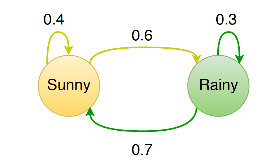Figure 1 shows a Markov chain for assigning a probability to a sequence of weather events. For example, \(p(\text{Sunny} \vert \text{Sunny}) = 0.4\) and \(p(\text{Rainy} \vert \text{Sunny}) = 0.6\). Notice that the outgoing probabilities of each state are normalized.

Formally speaking, a Markov chain can be defined as a tuple \((Q, A, q_0, q_F)\) where:

\(Q = q_{1}^{N} = q_1 q_2, \dots q_N\) is the set of N states
\[A = \begin{bmatrix} a_{01} & a_{02} & \dots & a_{0n} \\ a_{11} & a_{12} & \dots & a_{1n} \\ \vdots & \vdots & & \vdots \\ a_{n1} & a_{n2} & \dots & a_{nn} \\ \end{bmatrix}\]

is a transition probability matrix where \(a_{ij}\) represents the transition probability from state \(i\) to state \(j\) such that \(\sum_{j=1}^{n} a_{ij} = 1\) for all \(i \in \{0, \dots, N\}\). We have N+1 rows since we have N states and +1 for the special initial state \(q_0\).

\(q_0\) is a special label denoting the start or initial state (e.g \(\langle S \rangle\) for sentence start symbol)
\(q_F\) is a special label denoting the end state (e.g \(\langle E \rangle\) for sentence end symbol)

Now, if you want to think how the probability of the sequence of the Markov chain states looks like, you might think about something like this:

\[p(q_1, q_2, \dots, q_N) = \prod_i p(q_i \vert q_1, q_2, \dots, q_{i-1})\]

However, there is an important assumption known as the Markov process which the Markov chain follows. The idea is that the probability of the new state is only dependent on “part” of the history and not all of it. We say that the Markov chain is a first-order model if it only depends on the previous state and then the conditional probability becomes:

\[\big[p(q_i \vert q_1, q_2, \dots, q_{i-1}) = p(q_i \vert q_{i-1})\big] \implies p(q_1, q_2, \dots, q_N) = \prod_i p(q_i \vert q_{i-1})\]

Note that \(a_{ij} = p(q_j \vert q_i)\)

Note:

In some cases, a Markov chain can be defined differently where the initial and final states are explicitly defined. In this case, we will have the following components instead of \(q_0\) and \(q_F\):

\(\pi = \pi_{1} \pi_{2} \dots \pi_{N}\) where \(\pi_i\) is the probability that the model will start at state \(i\). This probability distribution over all the states is normalized and so \(\sum_{i=1}^{N} \pi_i = 1\)
\(Q_F \subseteq Q\) where \(Q_F\) is a set of final states

Exercise

Before you continue reading, try to compute the probability of the following sequences by referring to Figure 1 and assuming we have a first-order Markov chain model:

Sunny Sunny Sunny
Sunny Rainy Rainy

Hidden Markov Model

A Markov chain is usually used to compute the probability of a sequence of events that can be “observed” in the real world such as the weather example in Figure 1. However, in some cases, these observations are hidden (which represent the states) and that’s when we need to use HMMs. For example, when we have a sequence of words and we want to assign for each word its POS tag, then we do this by inference since the tags are hidden. HMM can be used for modelling the probability of both observed and hidden sequences.

First, let’s define HMM formally as we did for the Markov chain. HMM is defined as a tuple \((Q, A, O, B, q_0, q_F)\) where:

\(Q, A, q_0, q_F\) are defined same as the ones of the Markov chain above.
\(O = o_{1}^{T} = o_1 o_2 \dots o_T\) is a sequence of T observations drawn from some set \(V\)
\(B = p(o_t \vert q_i)\) is a sequence of observations likelihood also called emission probability. It represents the probability of generating observation \(o_t\) from state \(q_i\)

Note that in the case of Markov chain, the sequence of observations is represented by the states of the chain \(q_1 q_2 .. q_N\) and that’s why we didn’t define \(O\) (since they are observed and not hidden).

A first-order HMM has the following assumptions:

Markov assumption (same as Markov chain): the probability of a particular state depends only on the previous state

\[p(q_i \vert q_1, q_2, \dots, q_{i-1}) = p(q_i \vert q_{i-1})\]

Output Independence: the probability of an output observation \(o_t\) depends only on the state \(q_i\) that generated it and not on any other states or observations

\[p(o_i \vert q_1, \dots, q_i, \dots, q_T, o_1, \dots, o_i, \dots, o_T) = p(o_i \vert q_i)\]

Example:

Let’s consider again the chain of Figure 1 but now adding to it the initial and end states.

Figure 2: Hidden Markov chain

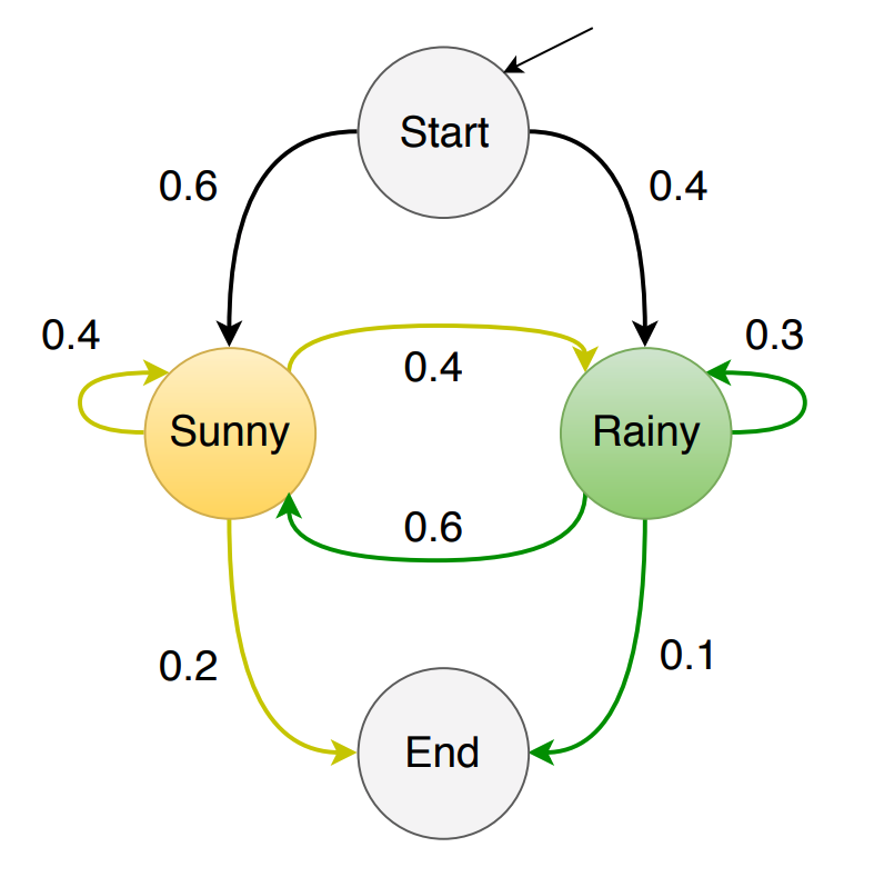Assume that the observations \(O = \{1, 2, 3\}\) correspond to the number of ice creams eaten on a given day and the hidden states are {Sunny, Rainy}. If for example let’s say the \(p(1 \vert Sunny) = 0.6\), then the joint probability of eating 1 ice cream in a Sunny day is \(p(1, Sunny) = p(\text{Sunny} \vert \text{Start}) \times p(1 \vert Sunny) = 0.6 \times 0.6 = 0.12\) where \(p(Sunny \vert Start)\) is known as the transition probability which is the probability of jumping from state Start to state Sunny. In addition, \(p(1 \vert Sunny)\) is known as the emission probability which is the probability of generating the observation 1 given state Sunny.

The questions that you might ask now are:

How to compute the emission probabilities?
How to compute the transition probabilities?
…

Hopefully, all your questions will be answered in the coming sections.

Fundamental problems:

The main problems that we are going to tackle next are:

Likelihood Computation: Given an HMM \(\mathcal{G}\) = (A, B) and an observation sequence \(O\), determine the likelihood probability \(p(O \vert G)\)
Decoding: Given an HMM \(\mathcal{G}\) = (A, B) and an observation sequence \(O\), compute the best hidden sequence \(Q\)
Training: Given a sequence of observations and set of states, learn the HMM parameters A and B

Likelihood Computation: The Forward Algorithm

Here we want to tackle the problem of computing the likelihood probability of an observation sequence. As for the ice cream example in the previous section, let’s say we have the following observation sequence (ice cream events) 3 1 1. Now, given the HMM \(\mathcal{G}\) = (A, B), we want to compute the likelihood probability which is \(p(O \vert \mathcal{G})\).

If we have a Markov chain, then the computation would be easy since the states represents the observations and so we can just follow the edges between the states and multiply the probabilities on them. However, when it comes to HMM, it is different. In HMM, the state sequence is hidden and so don’t know which path in the graph we have to take.

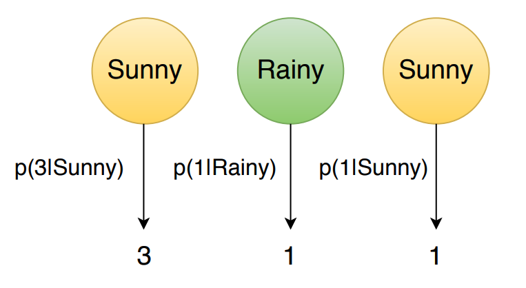
Let’s make the problem simpler. Suppose we know that the weather (hidden state sequence) would be Sunny Rainy Sunny. In addition, we know that there is a 1-1 mapping between the observations and the hidden states and the Markov assumption is used. Therefore, we can calculate the likelihood probability by just applying the chain rule as follows:

\[p(O \vert Q) = \prod_{i=1}^{T} p(o_i \vert q_i)\]

So, if we want to compute the forward probability for the given ice cream events, it would be:

\[p(3\ 1\ 1 \vert Sunny\ Rainy\ Sunny) = p(3 \vert Sunny) \times p(1 \vert Rainy) \times p(1 \vert Sunny)\]

where the values of the probabilities are assumed (for this problem) that they are given in \(\mathcal{G}\), in particular, by the parameter \(B\). Figure 3 represents this computation graphically.

Figure 3: Graphical representation of the likelihood computation of the ice cream events {3 1 1} given the hidden sequence {Sunny Rainy Sunny}

But here in our case, we just assumed some hidden sequence since we don’t know how this sequence looks like and there are other sequences that we need to consider. Thus, to compute the probability of the ice cream events 3 1 1, we need to sum over all the possible hidden (weather) sequences. To do so, let’s first compute the joint probability of being in a particular hidden (weather) sequence \(Q\) and generating a sequence \(O\) of ice cream events. For this, we have the following equation:

\[p(O, Q) = p(Q) \times p(O \vert Q) = \prod_{i=1}^{T} \underbrace{p(q_i \vert q_{i-1})}_{\text{transition probability}} \times \prod_{i=1}^{T} \underbrace{p(o_i \vert q_i)}_{\text{emission probability}}\]

To compute the joint probability of our example, we need to calculate the following equation:

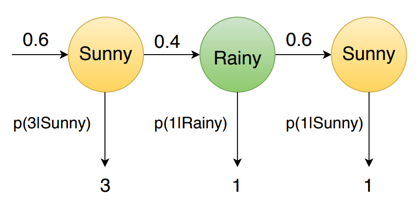
\[o(3\ 1\ 1, Sunny\ Rainy\ Sunny) = p(Sunny \vert Start) \times p(Rainy \vert Sunny) \times p(Sunny \vert Rainy) \times \\ \hspace{3.5cm} p(3 \vert Sunny) \times p(1 \vert Rainy) \times p(1 \vert Sunny)\]

The graphical representation is as follows,

Figure 4: Graphical representation of the joint probability computation of the ice cream events {3 1 1} given the hidden sequence {Sunny Rainy Sunny}

Now after knowing how to compute the joint probability, we can model the probability of an observation (likelihood) by summing over all the possible hidden sequences and so we get:

\[\begin{align} p(O) = \sum_{Q} p(O, Q) & = \sum_{Q} p(Q) \times p(O \vert Q) \\ & = \sum_{Q} \prod_{i=1}^{T} p(q_i \vert q_{i-1}) \times p(o_i \vert q_i) \hspace{1cm} [\text{First-order model}] \end{align}\]

We got the formula but can you see the problem? It is computationally expensive. In our example, we have N=2 hidden states {Sunny, Rainy} and an observation sequence of T=3 observations, then we have \(2^3\) possible hidden sequences since each observation can be generated by one of the N hidden states. Thus, the complexity is exponential which is \(\mathcal{O}(N^T)\). This is really not efficient since in real tasks N and T can be huge.

Here comes the help of Dynamic Programming (DP). The idea of DP is to store the solution for subproblems in a table and then use these values to build up the solution for the overall problem. Using DP, we can compute the above equation in an efficient \(\mathcal{O}(N^2 T)\) algorithm called the forward algorithm. It is called “forward” because we only do one forward pass over time (observation sequence).

Before formulating the DP problem, let’s first generalise how this works graphically.

Figure 5

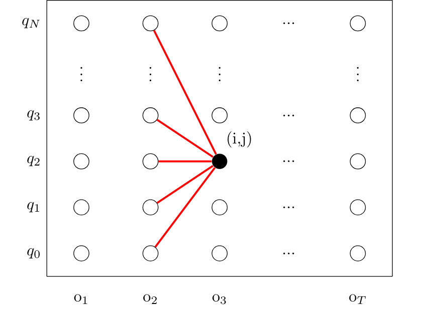I would think about this DP problem as what I drew in Figure 5. So, we have a Trellis which is a graph where nodes are ordered vertically over time. Each point \((i,j)\) in this graph represents a node where \(i\) represents the y-axis index and \(j\) represents the x-axis index. Then, each node would store the solution for the subproblem which is the “partial score up to this node”. So each node would store the score over all the paths that lead to this node which make sense now why we need only one forward pass :)

This is a generalised explanation about how to think about such DP problems to solve them. It can be used to solve different tasks also. In our case, we have the observation sequence of length T on the x-axis and the hidden states of the HMM of length N+2 (N states plus the start and end states) on the y-axis. I am going to use \(t\) for the time step index and \(q\) for state index just for meaning convenience.

Let’s now go into the mathematical details of the DP formulation of this problem. Recall the formula that we want to compute:

\[p(O) = \sum_{Q} \prod_{i=1}^{T} p(q_i \vert q_{i-1}) \times p(o_i \vert q_i)\]

Let \(forward[t][q]\) be the sum of the probabilities of all paths that lead to the node at position \((t,q)\).

Thus,

Initialization: \(forward[1][q] = p(q \vert q_0) \times p(o_1 \vert q)\)
Inductive step: \(forward[t][q] = \sum_{q'} forward[t-1][q'] \cdot p(q \vert q') \cdot p(o_t \vert q)\)
Termination: \(forward[T][q_F] = \sum_{q} forward[T][q] \cdot p(q_F \vert q)\)

In other words, \(forward[t][q]\) stores the sum of all paths up to the nodes in the previous time step \(t-1\) multiplied by the transition probability of each of these nodes to the current node (state) \(q\) and the emission probability of generating the observation at time step \(t\) given the current node \(q\).

Then, the pseudo code of the forward algorithm is:

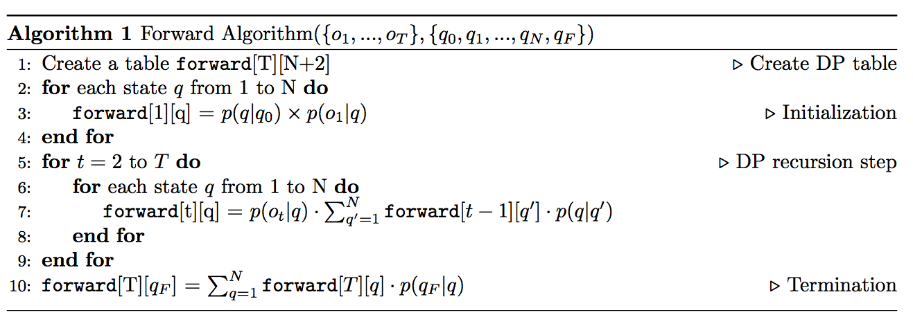Time Complexity: \(\mathcal{O}(N^2 T)\)

Space Complexity: \(\mathcal{O}(NT)\)

Decoding: The Viterbi Algorithm

To begin with, for such models, there is always a decoding task. Decoding means computing the best or most probable hidden sequence corresponding to a sequence of observations. In the ice cream example, given the observation sequence 3 1 1, the decoder job is to find the best hidden sequence consisting of the states {Sunny, Rainy}.

Now, a simple approach would be to apply the forward algorithm for each possible hidden sequence (Sunny Sunny Sunny, Sunny Rainy Sunny, etc) and then choose the one having the best (max) likelihood probability. However, this will be exponential and so computationally expensive.

To solve this problem efficiently, we need to somehow try to do only one pass over the observation sequence as we did before. In addition, you might have noticed that the main operation that we need here is “max” instead of “sum”. Then, the algorithm should be quite similar to the forward algorithm right? Try to think a bit how would you do it.

Therefore, we can use what’s called the Viterbi algorithm. It also uses dynamic programming to compute the result efficiently. So, formally speaking we have:

\[viterbi[t][q] = \max_{q_0, ..., q_{t-1}} p(q_0, q_1, ..., q_{t-1}, o_1, ..., o_t, q_t = q \vert \mathcal{G})\]

In other words, \(viterbi[t][q]\) is the probability of being in state \(q\) of the HMM after seeing \(t\) observations and passing through the best hidden sequence up to state \(q\).

Then, the calculation is:

Initialization: \(viterbi[1][q] = p(q \vert q_0) \times p(o_1 \vert q)\)
Inductive step: \(viterbi[t][q] = \max_{q'} viterbi[t-1][q'] \cdot p(q \vert q') \cdot p(o_t \vert q)\)
Termination: \(viterbi[T][q_F] = \max_{q} viterbi[T][q] \cdot p(q_F \vert q)\)

Thus, the pseudocode looks as follows:

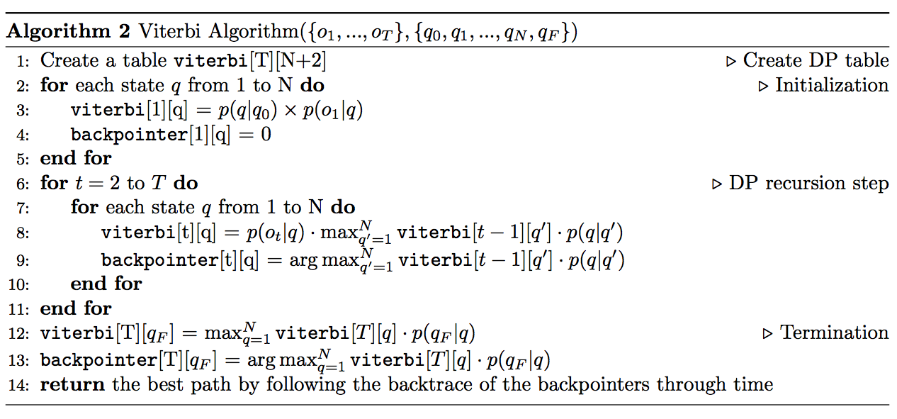Time Complexity: \(\mathcal{O}(N^2 T)\)

Space Complexity: \(\mathcal{O}(2NT)\)

Note that we have an extra table called \(backpointer\) in this algorithm. The reason why we need this table is because we want to be able to trace back the best path and so we use this table to store the index of the best previous state for each state at each time \(t\).

Training HMMs

Now we come to the last problem which is how to compute the parameters of the HMM. In particular, we want to compute the matrices A and B which represents the transition probabilities and emission probabilities respectively.

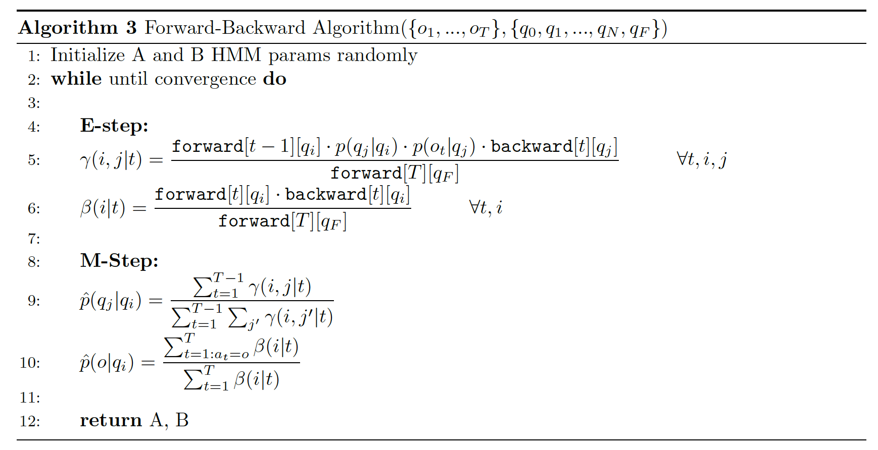
The input to the learning algorithm is an unlabeled sequence of observations and a set of hidden states. Since we have an unsupervised learning case, we need to use the Expected-Maximization algorithm (or EM algorithm). It is an iterative algorithm which works by computing an initial estimate for the probabilites we want to compute and then use these estimated to compute better probabilities and so on… Thus, training HMMs is done using what is known as the forward-backward, or Baum Welch algorithm which is a special case of the EM algorithm.

Concerning the learning of the transition probability, can you guess what would be a good estimate for the probability of going from state \(q_i\) to state \(q_j\)? Well, we can use counting:

\[p(q_j \vert q_i) = \dfrac{N(i, j)}{\sum_{j'} N(i, j')} \hspace{4cm} (Eq. 1)\]

where \(N(i, j)\) is the number of transitions from state \(q_i\) to state \(q_j\).

Now, if we have a Markov chain, then it would be easy to compute this estimation directly since we know the path that we need to follow because the states are seen. However, in the HMM case, we can’t do this easily. Therefore, we need to use the Baum Welch algorithm. The algorithm works by estimating the counts iteratively by starting with an initial estimate of the probabilities and then uses this estimate to compute better and better probabilities.

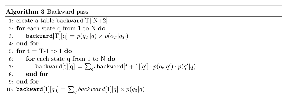
We already seen how we can do a forward pass and use dynamic programming to store the results so one part of the algorithm should be clear. Then, we still need to define the backward pass and how it is done. First, let

\[backward[t][q] = p(o_{t+1}, o_{t+2}, ..., o_T \vert q_t = q)\]

which stores the probability of seeing the observations from time \(t+1\) till the end, given that we are in state \(q\) at time step t. Now, let’s formulate the DP inductively as follows:

Initialization: \(backward[T][q] = p(q_F \vert q)\)
Inductive step: \(backward[t][q] = \sum_{q'} backward[t+1][q'] \cdot p(q' \vert q) \cdot p(o_t \vert q')\)
Termination: \(backward[1][q_0] = \sum_{q} backward[1][q] \cdot p(q \vert q_0)\)

We are now ready to dig deep into the forward-backward algorithm.

Let \(a\) be an alignment function where \(a_t = i\) means that the observation \(o_t\) is aligned to hidden state \(q_i\)

First, let’s change a bit in equation 1 to have the following:

\[p(q_j \vert q_i) = \dfrac{\text{expected number of transtions from state}\ q_i\ \text{to state}\ q_j}{\text{expected number of transitions from state}\ q_i}\]

How do we compute the numerator? Let \(\gamma(i, j \vert t)\) be the probability of being in state \(q_i\) at time \(t\) and state \(q_j\) at time \(t+1\). More formally,

\[\gamma(i, j \vert t) = \dfrac{\sum_{a_{1}^{T} : a_{t-1} = i, a_{t} = j} p(o_{1}^{T}, q_{1}^{T})}{\sum_{i', j'} \sum_{a_{1}^{T} : a_{t-1} = i', a_{t} = j'} p(o_{1}^{T}, q_{1}^{T})}\]

Do derivations by focusing on the numerator:

\[\begin{align} \sum_{a_{1}^{T} : a_{t-1} = i, a_{t} = j} p(o_{1}^{T}, q_{1}^{T}) & = \sum_{a_{1}^{T} : a_{t-1} = i, a_{t} = j} \prod_{i=1}^{T} p(q_i \vert q_{i-1}) \times p(o_i \vert q_i) \\ & = \sum_{a_{1}^{t-1} : a_{t-1} = i} \prod_{i=1}^{t-1} p(q_i \vert q_{i-1}) \times p(o_i \vert q_i) \cdot \Big[ p(q_j \vert q_i) \cdot p(o_t \vert q_j) \Big] \cdot \\ & \sum_{a_{t+1}^{T} : a_{t} = j} \prod_{i=t+1}^{T} p(q_i \vert q_{i-1}) \times p(o_i \vert q_i) \\ & = forward[t-1][q_i] \cdot \Big[ p(q_j \vert q_i) \cdot p(o_t \vert q_j) \Big] \cdot backward[t][q_j] \end{align}\]

Therefore,

\[\gamma(i, j \vert t) = \dfrac{forward[t-1][q_i] \cdot \Big[ p(q_j \vert q_i) \cdot p(o_t \vert q_j) \Big] \cdot backward[t][q_j]}{\sum_{i', j'} forward[t-1][q_{i'}] \cdot \Big[ p(q_{j'} \vert q_{i'}) \cdot p(o_t \vert q_{j'}) \Big] \cdot backward[t][q_{j'}]}\]

Then, the expected number of transitions from state \(q_i\) to state \(q_j\) is then the sum over all \(t\) of \(\gamma\).

\[\hat{p}(q_j \vert q_i) = \dfrac{\sum_{t=1}^{T-1} \gamma(i, j \vert t)}{\sum_{t=1}^{T-1} \sum_{j'}\gamma(i, j' \vert t)}\]

Next, we need to estimate the emission probabilities so we have:

\[p(o \vert q_i) = \dfrac{\text{expected number of times of seeing}\ o\ \text{while being in state}\ q_j}{\text{expected number of times of being in state}\ q_i}\]

We do as before by defining the probability \(\beta(i \vert t)\) which is the probability of being in state \(q_i\) at time step \(t\). More formally,

\[\beta(i \vert t) = \dfrac{\sum_{a_{1}^{T} : a_t = i} p(o_{1}^{T}, q_{1}^{T})}{\sum_{i'} \sum_{a_{1}^{T} : a_t = i'} p(o_{1}^{T}, q_{1}^{T})}\]

Apply some derivations:

\[\begin{align} \sum_{a_{1}^{T} : a_t = i} p(o_{1}^{T}, q_{1}^{T}) & = \sum_{a_{1}^{T} : a_t = i} \prod_{i=1}^{T} p(q_i \vert q_{i-1}) \times p(o_i \vert q_i) \\ & = \Big[\sum_{a_{1}^{t} : a_t = i} \prod_{i=1}^{t} p(q_i \vert q_{i-1}) \times p(o_i \vert q_i) \Big] \cdot \Big[ \sum_{a_{t+1}^{T} : a_t = i} \prod_{i=t+1}^{T} p(q_i \vert q_{i-1}) \times p(o_i \vert q_i) \Big] \\ & = forward[t][q_i] \cdot backward[t][q_i] \end{align}\]

Therefore,

\[\beta(i \vert t) = \dfrac{forward[t][q_i] \cdot backward[t][q_i]}{\sum_{i'} forward[t][q_{i'}] \cdot backward[t][q_{i'}]}\]

and,

\[\hat{p}(o_t \vert q_i) = \dfrac{\sum_{t=1 : a_t = i}^{T} \beta(i \vert t)}{\sum_{t=1}^{T} \beta(i \vert t)}\]

Finally, here is the pseudocode of the forward-backward algorithm:

Written on October 7, 2018