Let's Pay Attention

Introduction

Statistical machine translation was the main approach used for machine translation before neural networks become popular. These models are composed of different statistical models where each would be trained separately thus probably lacking a global optimization. However, nowadays, everything can be trained in a single neural network by jointly tuning it to maximize the translation performance. These models are known as sequence-to-sequence models (or seq2seq) since the input is a source sequence and the output is a target sequence. For example, for the translation task the input and output can be sequence of words. In general, the models proposed recently for machine translation are represented as an encoder-decoder architecture where the source sentence is “encoded” in a fixed vector which represents somehow its context, and then the decoder “decodes” or generates the target sentence using this encoded vector.

These seq2seq models are also applied for other tasks such as Automatic Speech Recognition but I am going to focus on the machine translation task in this blog post since the main papers about attention, which is the main topic of this blog post, are published in the machine translation papers.

The main paper which I am going to follow is Neural Machine Translation by Jointly Learning to Align and Translate. The idea is that using the encoder’s fixed vector can lead to some problems in improving the translation task and so instead of that, we allow the decoder to (softly) attend to some of the parts of the source sentence that are mostly related to the word we want to translate to. To make things more clear, I am going first to explain briefly how recurrent neural networks work since it is a main component in these models. Then, I am going to talk about the encoder-decoder architecture and what are its problems. After that, I am going to introduce the Attention model which lead to a huge improvement in the performance of these models. In the end, we look at some experiments and results.

Recurrent Neural Network (RNN)

The idea here is that we want to save/use the past information for the incoming outputs. For example, if you are reading a text, you will not each time start thinking from scratch but understand what are you reading depending on what you read before.

It is not clear how standard neural networks can do this and that’s why we need recurrent neural networks. In addition to that, here we have a sequence of inputs and outputs with variable lengths. To address these issues, RNN has some form of loop which allows the persistence of the information. A simple architecture of an RNN looks as follows:

Figure 1: RNN Architecture. Source: [2]

In Figure 1, the most left image represents a general form of an RNN which can be unfolded into multiple copies to get what is shown on the right side. In other words, at each time step \(t\), one input is fed to the network to produce an output. The labels of the network are:

\(x_t\): Input at time step \(t\). For example, it can be a one-hot vector representing the index of an input word.
\(h_t\): Hidden state at time step \(t\). The context is saved in this hidden state so it represents the memory of the network.
\(o_t\): Output at time step \(t\). For example, it can be a one-hot vector representing the index of the translated word of the input word.
\(U, V, W\): Weight matrices parameters. U is the input-to-hidden weight matrix, V is the hidden-to-hidden weight matrix, and W is the hidden-to-output weight matrix. Note that these matrices are shared between all the time steps in the network.

The loop allows information to pass from one step to another. For the calculations:

\(h_t = g[Ux_t + Vh_{t-1}]\) where the current hidden state or information is calculated depending on the current input and the previous information. \(g\) is an activation function.
\(o_t = Softmax(Wh_t)\). Since we are dealing with a translation task, then the output would be a vector of probabilities across the vocabulary words.

However, usually the hidden state \(h_t\) is not able to capture a lot of information for long sequences and so to decrease the impact of this problem, Long-Short-Term-Memory (LSTMs) are used. I will explain briefly how LSTMs work since they are not so important for understanding the attention model and so you can skip it. But, if you want to know more about them, I recommend to check colah’s blog.

LSTM uses gates to control the flow of information through what is called a cell state which is denoted by \(c_t\) for each time step of the network. The LSTM hidden state receives input \(x_t\) and the previous hidden state \(h_{t-1}\):

\[h_t = W_{hh}h_{t-1} + W_{hx}x_t\]

where \(W_{hh}\) is the hidden-to-hidden weight matrix, and \(W_{hx}\) is the input-to-hidden weight matrix. Then, LSTM uses the following three gates:

Forget gate: \(\hspace{0.3cm} f_t = \sigma(W_{fx}x_t + W_{fh}h_{t-1})\)

Input gate: \(\hspace{0.5cm} i_t = \sigma(W_{ix}x_t + W_{ih}h_{t-1})\)

Output gate: \(\hspace{0.2cm} o_t = \sigma(W_{ox}x_t + W_{oh}h_{t-1})\)

where \(\sigma\) is a sigmoid function. The forget gate determines how much of the previous cell state \(c_{t-1}\) we want to forget. The input gate controls how much of the input to each hidden unit is written to the cell state \(c_t\). The output gate controls how much of the output of each hidden unit is preserved. In other words, this allows the LSTM hidden unit to store information which are currently important and store the rest in the cell state which can be used later. Therefore, we end up with the following equations:

\[c_t = f_t \odot c_{t-1} + i_t \odot tanh(h_t)\]

Since \(f_t\) uses sigmoid, we apply a Hadamard product with \(c_{t-1}\) to forget unnecessary information and then we add the result to the hidden unit output.

\[h_t = tanh(c_t) \odot o_t\]

Bidirectional RNN

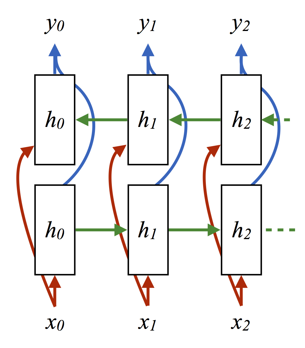
As discussed in the previous section, each hidden state can be considered as a memory that capture the context information in each time step \(t\). This is known as a unidirectional RNN since the information flow is in one direction from left to right, and in particular, from the start to the end of the sequence. But what if we want the information at some time \(t\) to be from both the past and future context? Therefore, we use what is called a Bidirectional RNN (BRNN). It has the same architecture as a unidirectional RNN but with two layers of hidden states instead. The first layer will contain the forward pass information flow and the other layer will contain the backward pass information flow. To illustrate more, here how the architecture looks like now:

Figure 2: BRNN Architecture. Source: [3]

In Figure 2, the hidden state at time step \(t\) is then \(h_t = \begin{bmatrix} \overrightarrow{h_t} \\ \overleftarrow{h_t} \end{bmatrix}\) which is the concatenation of the forward and backward hidden states. In this way, we have information flow from both past and future context.

Encoder-Decoder Architecture

Most of the neural machine translation models belong to a family of encoders and decoders.

Figure 3: Encoder-Decoder Architecture. Source: [4]

Figure 3 shows the encoder-decoder architecture in general.

For machine translation, an RNN encoder-decoder is used and so the encoder reads the input sequence \(X = (x_1, ..., x_{T_x})\), where \(T_x\) is the number of time steps and \(x_t\) is the input vector at time step \(t\), and then encodes it into a fixed-size vector \(c\).

\[h_t = f(x_t, h_{t-1})\ \text{and}\ c = g(\{h_1, ..., h_{T_x}\})\]

where \(f\) and \(q\) are nonlinear functions. For example, \(f\) can be an LSTM and \(g(\{h_1, ..., h_{T_x}\})\) can be just the last hidden state which is \(h_{T_x}\).

Now, after computing the context vector \(c\), the decoder is trained to predict the next word \(y_{t'}\) in the target sequence given this context vector and all the previous predicted outputs \(\{y_1, y_2, ..., y_{t'-1}\}\). Thus, the decoder is trained to maximize the following probability:

\[p(Y) = \prod_{t'=1}^{T_y} p(y_{t'} \vert \{y_1, ..., y_{t'-1}\}, c)\ \text{where}\ Y = (y_1, ..., y_{T_y})\]

Since we are dealing with an RNN, then \(p(y_{t'} \vert \{y_1, ..., y_{t'-1}\}, c) = A(y_{t-1}, s_t, c)\) where \(A\) can be a multilayer feed-forward network to calculate the output \(y_t\) depending on the previous output \(y_{t-1}\), the decoder’s hidden state at time step t \(s_t\), and the context vector \(c\). These calculations are represented graphically in Figure 4.

Figure 4: RNN Encoder-Decoder Architecture. Source: [5]

Note that the total number of time steps of the encoder and decoder are not the same and that is why they are distigushed since the source and target sentences can have different lengths.

Attention Model

Before talking about the main part of this blog post, let’s first answer the question what is the motivation behind this model and what are the problems of the RNN encoder-decoder architecture discussed in the previous section. The main problem with this encoder-decoder approach is that the neural network should be capable somehow to store all the necessary information of the source sentence and encode it in this context vector. However, this can be problematic for long sentences especially for the ones that are longer than the sentences in the training corpus.

Thus, we need a mechanism that allows us to “attend” only to the parts of the encoder that we think they are important for the prediction of the current next word. So now the neural network doesn’t need to encode all the information of the source sentence into one fixed-size vector but instead chooses a subset of the encoder hidden states vectors and encodes them adaptively while decoding. This mechanism is called “Learning to Align and Translate” since this is done jointly while decoding. The word “align” refers to the attention model since we are aligning the decoder hidden state \(s_t\) to the encoder hidden states \(\{h_1, ..., h_{T_x}\}\).

Learning to Align and Translate

For this section, I am going to use \(i\) for output step, and \(j\) for input step.

Figure 5: Model with Attention. Source: [1]

Encoder Architecture

In this model, we would like at each time step to capture information not only from the preceding words but also from the future ones. So for that we use a bidirectional RNN which is explained briefly before. In Figure 5, we have an input sequence \((x_1, ..., x_{T})\). Then, the forward RNN reads the input sequence from \(x_1\) to \(x_T\) and outputs a vector of forward hidden states for each time step: \((\overrightarrow{h_1}, ..., \overrightarrow{h_T})\). In addition, the backward RNN reads the input sequence from \(x_T\) to \(x_1\) resulting in a sequence of backward hidden states: \((\overleftarrow{h_1}, ..., \overleftarrow{h_T})\). Then, at each time step we concatenate these calculated hidden states and so \(h_j = \begin{bmatrix} \overrightarrow{h_j} \\ \overleftarrow{h_j} \end{bmatrix}\)

Decoder Architecture

So now each decoder hidden state \(s_i\) depends on a context vector \(c_i\) instead of a fixed vector. Thus, let’s first define the new probability of the decoder’s output:

\[p(y_i \vert y_1, ..., y_{i-1}, c_i) = A(y_{i-1}, s_i, c_i)\]

Moreover, the context vector \(c_i\) depends on a sequence of encoder hidden states \((h_1, ..., h_{T_x})\) to which the encoder maps the input sequence. Each \(h_j\) contains information about the whole sequence (since we are dealing with an RNN), with a focus on the surrounding parts at position \(j\) (because of the BRNN).

The context vector can be computed as follows:

\[c_i = \sum_{j = 1}^{T_x} \alpha_{ij} h_j\]

The weight \(\alpha_{ij}\) of each hidden state \(h_j\) is computed by

\[\alpha_{ij} = Softmax(e_i) = \dfrac{\exp(e_{ij})}{\sum_{k=1}^{T_x} \exp(e_{ik})}\]

where \(e_{ij} = a(s_{i-1}, h_j)\) is known as the energy score.

To explain what is happening in the above equations, let’s first consider the computation of the context vector. So as I mentioned earlier, the context vector depends on parts of the encoder hidden states and so its computation depends on a weighted linear combination of all states. The weights are denoted as \(\alpha_{ij}\) which represents how much \(s_i\) is related to \(h_j\). Now, to compute these weights, we need to define a “score” function \(a\) that takes as input \(s_i\) and \(h_j\). We can have the following score functions:

\[a(s_{i}, h_{j}) = \begin{cases} h_{j}^{T}s_i & dot \\ h_{j}^{T} W_a s_i & general \\ v_{a}^T tanh (W_a[h_j;s_i]) & concat \end{cases}\]

In theory, all these functions should be almost the same, however, they usually differ in practice. The first case is known as “dot attention” which is simply a vector similarity. The second case is proposed by Stanford in [6] where the weight matrix \(W_a\) is trained to somehow capture the relation between the two states. The third case is known as “additive attention” which is a one layer feed-forward neural network. \(v_a\) is a trained vector which is used to get a scalar energy score since the \(tanh\) would output a vector. I think dot attention would be the faster one in practice. This is also known as the alignment model since we are aligning each decoder state to a subset of the encoder states.

Now after computing the energy scores, it is time to compute the weights. For that, we use a Softmax function where the input is a vector of energy scores between \(s_i\) and \(h_j\) for all \(j\).

Note that in the original paper [1] the energy scores are dependent on the previous hidden state \(s_{i-1}\) instead of \(s_i\), but in [6], they used \(s_i\).

Experiments

The experiments are performed on the task of English-to-French translation. The dataset used is WMT ‘14. The BLUE score [7] is usually used as the metric for the translation performance measure. The idea of BLUE is that the similar the machine translation to a professional human translation the better. So given a candidate or hypothesis translation and a set of reference translations (human translations) then to compute the score, we calculate what is called the modified n-gram precision by comparing the n-grams between the hypothesis and the references. The position is independent and it is called “modified” precision because a reference word will be marked as visited after a match so that it is not matched again. For example, if we have a hypothesis sentence: the the the and reference sentence: the cat, the modified precision is equal to 1/3 and not 3/3.

Figure 6: The BLUE scores of the generated translations on the test dataset. Source: [1]

Figure 6 shows how attention can solve the problem of long sentences. RNNenc is an RNN Encoder-Decoder model and RNNsearch is the same but with attention. The number in the suffix represents the max length of the sentences in the training dataset. We can see that for long sentences, the BLUE score is stable when using attention, but it decreases rapidly without it.

Just to note that for decoding, we use what is called “Beam Search” algorithm. I am not going to go into the details of this algorithm but the idea is that a greedy search approach for the next word won’t result in the optimal output. Therefore, we define a beam (e.g stack) of size B and each time while decoding, we choose the best B hypotheses and add them to the beam. After that, we model the next conditional probability for each word given only these hypotheses and continue until we reach the end sentence symbol.

Figure 7: Attention weights illustration. Source: [1]

Figure 7 highlights the alignment model and more precisely how the attention weights are computed for each target word. We want to translate the english source sentence into a target french sentence. The alignment looks monotonic where most of the weights are high on the diagonal of the matrix. There are some non-monotonic alignments which refers to the reordering of Adjectives and nouns between French and English.

References

Written on August 29, 2018